Quantum Search Algorithm (Full)

Full-length article on Grover's Algorithm, i.e. Quantum Search Algorithm, which efficiently searches an unsorted database.

Posted Mar 13, 2025 Updated Feb 28, 2026

Quantum circuit representation of Grover's algorithm generated by Qiskit

By Kiran Brahmatewari

13 min read

Quantum Search Algorithm (Full)

This is a full-length article on Grover’s algorithm. For a shorter version, see Quantum Search Algorithm.
The contents of this article have been taken from my Jupyter notebook on Grover’s Algorithm, which can be found in my repository.
There’s also an accompanying Python script, if you prefer.

Constants

$n$, SHOTS $\in \mathbb{Z^{+}}$

OPTIMIZATION_LEVEL $\in \{ 0, 1, 2, 3 \}$

SEARCH_VALUES $\subseteq \{\,x \in \mathbb{W} \mid 0 \le x \lt 2^{n}\,\}$

  
from qiskit import QuantumRegister

"""Number of qubits."""
N: int = 4

"""N-qubit quantum register."""
QUBITS: QuantumRegister = QuantumRegister(N, "qubit")

"""Set of m nonnegative integers to search for using Grover's algorithm (i.e. TARGETS in base 10)."""
SEARCH_VALUES: set[int] = { 9, 0, 3 }

"""Set of m N-qubit binary strings representing target state(s) (i.e. SEARCH_VALUES in base 2)."""
TARGETS: set[str] = { f"{s:0{N}b}" for s in SEARCH_VALUES }

"""Amount of times to simulate the algorithm."""
SHOTS: int = 10000

"""How much optimization to perform on the circuits.
   Higher levels are more optimized, but take longer to transpile.

   * 0 = No optimization
   * 1 = Light optimization
   * 2 = Heavy optimization
   * 3 = Heavier optimization
"""
OPTIMIZATION_LEVEL: int = 2

"""Title"""
TITLE: str = f"Outcome of {SHOTS} simulations of Grover's algorithm"

Oracle

Oracle $U_{w}$ flips the sign(s) of $n$-qubit target state(s) while leaving all other orthogonal states unchanged.

$U_{w} = X(MCZ)X$

Pauli-X gate $X$ is applied to qubit $\ket{q_{i}}$ if $q_{i} = 0$ in target state $\ket{q_{n - 1}, \ldots, q_{0}}$. After $X$ is applied to the appropriate qubit(s), target state is transformed to $\ket{1}^{\otimes n}$. Then $(n − 1)$-control Z gate $MCZ$ flips the sign of $\ket{1}^{\otimes n}$.

We simulate $MCZ$ by applying Hadamard gate $H$, $(n - 1)$-control Toffoli gate $MCT$, and another $H$ to qubit $\ket{q_{n - 1}}$

$MCZ = H(MCT)H$

Finally, $X$ is applied again to the appropriate qubit(s) to reverse the transformation by the first $X$. This entire process is applied to all target state(s), which we’ve implemented in oracle():

$U_{w} = XH(MCT)HX$

  
from qiskit import QuantumCircuit

def flip(target: str, qc: QuantumCircuit, qubit: str = "0") -> None:
    """Flips qubit in target state.

    Args:
        target (str): Binary string representing target state.
        qc (QuantumCircuit): Quantum circuit.
        qubit (str, optional): Qubit to flip. Defaults to "0".
    """
    for i in range(len(target)):
        if target[i] == qubit:
            qc.x(i) # Pauli-X gate
            
def oracle(targets: set[str] = TARGETS, qubits: QuantumRegister = QUBITS, name: str = "Oracle") -> QuantumCircuit:
    """Mark target state(s) with negative phase.

    Args:
        targets (set[str]): Binary string(s) representing target state(s). Defaults to TARGETS.
        name (str, optional): Quantum circuit's name. Defaults to "Oracle".

    Returns:
        QuantumCircuit: Quantum circuit representation of oracle.
    """
    # Create N-qubit quantum circuit for oracle
    oracle = QuantumCircuit(qubits, name = name)

    for target in targets:
        # Reverse target state since Qiskit uses little-endian for qubit ordering
        target = target[::-1]
        
        # Flip zero qubits in target
        flip(target, oracle, "0")

        # Simulate (N - 1)-control Z gate
        oracle.h(N - 1) # Hadamard gate
        oracle.mcx(list(range(N - 1)), N - 1) # (N - 1)-control Toffoli gate
        oracle.h(N - 1) # Hadamard gate

        # Flip back to original state
        flip(target, oracle, "0")

    return oracle

# Generate and display oracle
grover_oracle = oracle(TARGETS, name = "Oracle")
grover_oracle.draw("mpl", style = "iqp")

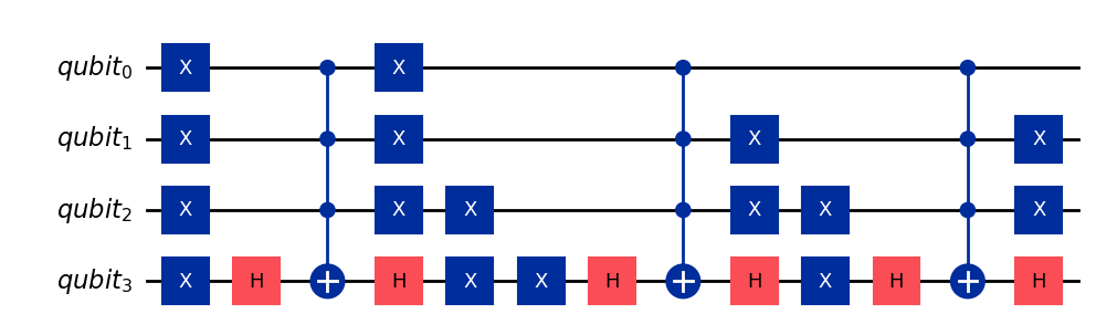Generated quantum circuit for Oracle

Diffuser

Diffuser $D$ amplifies the target state(s) (which deamplifies all other states) with a reflection about the average amplitude. In other words, it increases the probability of getting the $n$-qubit target state(s) marked by $U_{w}$ and, ultimately, the right answer.

$D = H^{\otimes n}U_{0}H^{\otimes n}$

We create $D$ by applying $H^{\otimes n}$, $U_{w}$ with its target state $w$ set to $\ket{0}^{\otimes n}$, and $H^{\otimes n}$ again to each qubit. This leaves us with the final equation we’ve implemented in diffuser():

  
def diffuser(name: str = "Diffuser") -> QuantumCircuit:
    """Amplify target state(s) amplitude, which decreases the amplitudes of other states and increases the probability of getting the correct solution (i.e. target state(s)).

    Args:
        name (str, optional): Quantum circuit's name. Defaults to "Diffuser".

    Returns:
        QuantumCircuit: Quantum circuit representation of diffuser (i.e. Grover's diffusion operator).
    """
    # Create N-qubit quantum circuit for diffuser
    diffuser = QuantumCircuit(QUBITS, name = name)
    
    # Hadamard gate
    diffuser.h(QUBITS)

    # Oracle with all zero target state
    diffuser.append(oracle({ "0" * N }), list(range(N)))

    # Hadamard gate
    diffuser.h(QUBITS)
    
    return diffuser

# Generate and display diffuser
grover_diffuser = diffuser()
grover_diffuser.draw("mpl", style = "iqp")

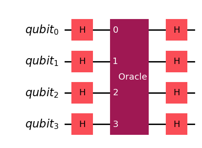Generated quantum circuit for Diffuser

Grover’s Algorithm

Grover’s algorithm, also known as quantum search algorithm, finds $m$ target(s) within a database of size $N$; this is particularly useful for unstructured searches. A search is performed by evaluating a function (i.e. $U_{w}$) that returns a particular value for the target(s) and another value for all other objects in the database. More generally, it solves the problem of function inversion: Given $y = f(x)$ where $x$ can take $N$ values, Grover’s algorithm finds the value $x = f^{−1}(y)$ with $O(\sqrt{N})$ evaluations; a naïve exhaustive search (i.e. classical algorithm) would require about $O(N)$ evaluations. This is a significant, quadratric speed-up!

$m, N \in \mathbb{Z^{+}}$

The first step of the algorithm involves encoding all objects of the database as orthogonal states. That is, initializing all $n$ qubits to $\ket{0}$. Assuming maximum uncertainty about the $n$-qubit target state(s), the initial state is chosen to be the uniform superposition $\ket{s}$ of all basis states:

$\ket{s} = (H \ket{0})^{\otimes n}$

We do this by applying $H$ on all qubits. Afterwards, we increase the likelihood of detecting the target state(s) at the end by applying $U_{w}$ followed by $D$ (also known as Grover operator) to $\ket{s}$ an optimal amount of times $t$. After $t$ iterations, the state(s) will have transformed to $\ket{\psi_{t}}$:

$\ket{\psi_{t}} = (DU_{w})^{t} \ket{s}$

Where:

$t \in \mathbb{Z^{+}}$

$t \approx \lfloor \frac{\pi}{4} \sqrt{\frac{N}{m}}\rfloor$

In this case, $N = 2^{n}$, so $t$ can be simplified:

$t \approx \lfloor \frac{\pi}{4} \sqrt{\frac{2^{n}}{m}}\rfloor$

The final step involves measuring $\ket{\psi_{t}}$, which should return the target state(s) with near-certainty (i.e. probability very close to $1$).

  
from math import pi, sqrt
from qiskit.quantum_info import DensityMatrix

def grover(oracle: QuantumCircuit = oracle(), diffuser: QuantumCircuit = diffuser(), name: str = "Grover Circuit") -> tuple[QuantumCircuit, DensityMatrix]:
    """Create quantum circuit representation of Grover's algorithm,
    which consists of 4 parts: (1) state preparation/initialization,
    (2) oracle, (3) diffuser, and (4) measurement of resulting state.
    
    Steps 2-3 are repeated an optimal number of times (i.e. Grover's
    iterate) in order to maximize probability of success of Grover's algorithm.

    Args:
        oracle (QuantumCircuit, optional): Quantum circuit representation of oracle. Defaults to oracle().
        diffuser (QuantumCircuit, optional): Quantum circuit representation of diffuser. Defaults to diffuser().
        name (str, optional): Quantum circuit's name. Defaults to "Grover Circuit".

    Returns:
        tuple[QuantumCircuit, DensityMatrix]: Quantum circuit representation of Grover's algorithm and its density matrix.
    """
    # Create N-qubit quantum circuit for Grover's algorithm
    grover = QuantumCircuit(QUBITS, name = name)

    # Intialize qubits with Hadamard gate (i.e. uniform superposition)
    grover.h(QUBITS)
    
    # Apply barrier to separate steps
    grover.barrier()
    
    # Apply oracle and diffuser (i.e. Grover operator) optimal number of times
    for _ in range(int((pi / 4) * sqrt((2 ** N) / len(TARGETS)))):
        grover.append(oracle, list(range(N)))
        grover.append(diffuser, list(range(N)))

    # Generate density matrix representation of Grover's algorithm
    density_matrix = DensityMatrix(grover)

    # Measure all qubits once finished
    grover.measure_all()
    
    return grover, density_matrix

# (1) Generate and display quantum circuit for Grover's algorithm, and (2) Get density matrix
grover_circuit, density_matrix = grover(grover_oracle, grover_diffuser)
grover_circuit.draw("mpl", style = "iqp")

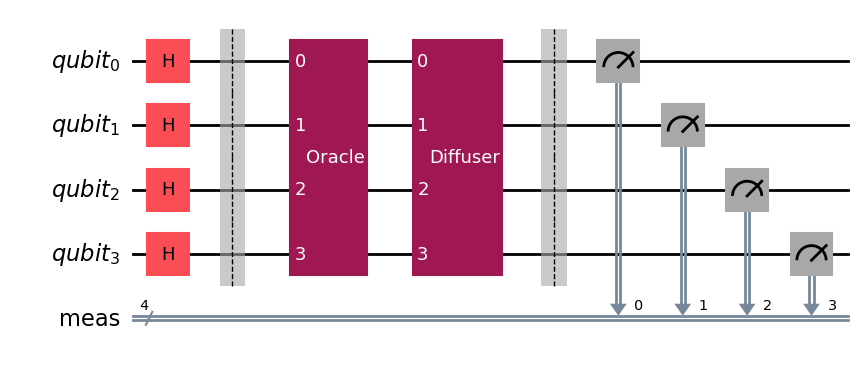Generated quantum circuit for Grover’s algorithm

Here we simulate Grover’s algorithm using the AerSimulator backend, which is a local simulator that can simulate quantum circuits with noise. We transpile the circuit to optimize it for the backend, then run the simulation with a specified number of shots. We then get the results of the simulation and display the top measurement(s) (state(s) with the highest frequency) and target state(s) in binary and decimal form. We determine if the top measurement(s) equals the target state(s) and print the result.

  
from heapq import nlargest
from qiskit import transpile
from qiskit_aer import AerSimulator

# Simulate Grover's algorithm locally
backend = AerSimulator(method = "density_matrix")

# Transpile circuit
transpiled = transpile(grover_circuit, backend, optimization_level = OPTIMIZATION_LEVEL)

# Display transpiled circuit
transpiled.draw("mpl", style = "iqp")

# Run simulation 
simulation = backend.run(transpiled, shots = SHOTS)

# Get results
results = simulation.result().get_counts()

# State(s) with highest count and their frequencies
winners = { winner : results.get(winner) for winner in nlargest(len(TARGETS), results, key = results.get) } # type: ignore

def outcome(winners: list[str], counts) -> None:
    """Print top measurement(s) (state(s) with highest frequency)
    and target state(s) in binary and decimal form, determine
    if top measurement(s) equals target state(s), then print result.

    Args:
        winners (list[str]): State(s) (N-qubit binary string(s))
        with highest probability of being measured.
        counts (Counts): Each state and its respective frequency.
    """
    print("WINNER(S):")
    print(f"Binary = {winners}\nDecimal = {[ int(key, 2) for key in winners ]}\n")
        
    print("TARGET(S):")
    print(f"Binary = {TARGETS}\nDecimal = {SEARCH_VALUES}\n")

    if not all(key in TARGETS for key in winners): print ("Target(s) not found...")

    else:
        winners_frequency, total = 0, 0

        for value, frequency in counts.items():
            if value in winners:
                winners_frequency += frequency
            total += frequency
        
        print(f"Target(s) found with {winners_frequency / total:.2%} accuracy!")

# Print outcome
outcome(list(winners.keys()), results)

WINNER(S):
Binary = ['0011', '1001', '0000']
Decimal = [3, 9, 0]

TARGET(S):
Binary = {'0000', '0011', '1001'}
Decimal = {0, 9, 3}

Target(s) found with 94.99% accuracy!

Finally, we display the simulation results as a histogram. The histogram shows the frequency of each state measured during the simulation. The state(s) with the highest frequency are the winner(s) and should equal the target state(s).

  
from qiskit.visualization import plot_histogram

# Display simulation results as histogram
plot_histogram(data = results, legend = ["Qubits"], number_to_keep = len(TARGETS), title = TITLE)

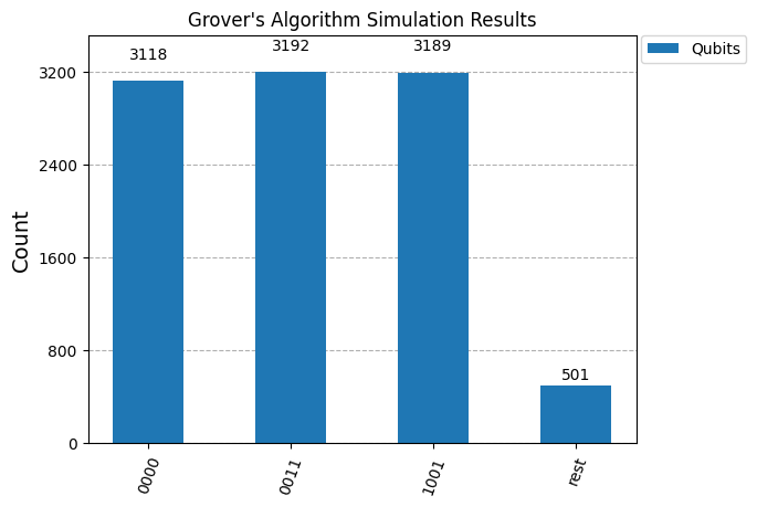Simulation results of Grover’s algorithm

Density Matrix

Density matrix is a collection of numbers in a matrix used to describe $n$-qubit state(s) in a system. In our case, density_matrix represents $m$ winner(s) (which should equal our target state(s)), and is visualized in the diagrams below.

City Plot

City plot is made up of two 3D bar graphs representing the real and imaginary parts of an $n$-qubit state. Each bar’s length is proportional to the magnitude of the corresponding number.

  
# City plot of density_matrix
density_matrix.draw("city")

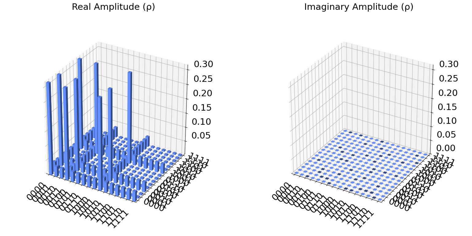City plot representation of density matrix

Bloch Sphere

Bloch sphere is a 3D geometric representation of a single qubit’s state. A point $(\theta, \phi)$ on the sphere’s surface denotes a pure state, represented by state vector $\ket{\psi}$, with its north and south poles corresponding to $\ket{0}$ and $\ket{1}$ respectively. This means that we can always say for certain (100% probability) that our system’s in state $\ket{\psi}$. In other words, for a pure state we have complete knowledge of the system and know exactly what state it’s in.

$\ket{\psi} = \alpha \ket{0} + \beta \ket{1}$

Probability amplitudes $\alpha$ and $\beta$ can be real or complex numbers.

$\alpha = cos(\frac{\theta}{2})$

$\beta = e^{i \phi} sin(\frac{\theta}{2})$

$\theta, \phi \in \mathbb{R}$ where $0 \le \theta \le \pi$ and $0 \le \phi \le 2\pi$.

The probability of obtaining $\ket{0}$ and $\ket{1}$ after measurement is $\vert \alpha \vert^{2}$ and $\vert \beta \vert^{2}$ respectively, hence the total probability of the system being observed in $\ket{0}$ or $\ket{1}$ is $1$:

$\vert \alpha \vert^{2} + \vert \beta \vert^{2} = 1$

A point inside the sphere denotes a mixed state, represented by density matrix $\hat{\rho}$, which is a probability distribution of different pure states, with a maximally mixed state at the sphere’s center (equal probabilities of being observed in $\ket{0}$ or $\ket{1}$). $\hat{\rho}$ is a generalized version of a state vector and is used to represent the system when we’re uncertain of its state.

$\hat{\rho} = \sum\limits_{k}^{N} p_{k} \ket{\psi_{k}} \bra{\psi_{k}} = \displaystyle\frac{1}{2} \begin{bmatrix}1 + r_{z} & r_{x} - ir_{y} \ r_{x} + ir_{y} & 1 - r_{z}\end{bmatrix}$

Weights $p_{k}$ can be interpreted as the probability of the system being in state $\ket{\psi_{k}}$ where $0 \le p_{k} \le 1$. Note: $\hat{\rho}$ of a pure state naturally reduces to $\ket{\psi}$ with $p = 1$.

$N$ is the total number of possible states the system could be in with $\sum\limits_{k}^{N} p_{k} = 1$.

$\ket{\psi_{k}} \bra{\psi_{k}}$ represents the outer product of the state $\ket{\psi_{k}}$ with itself, producing a matrix known as the projection operator $\hat{P_{\psi_{k}}}$.

Coefficients $r_{x}, r_{y}, r_{z}$ are components of the vector representing a mixed state, known as the Bloch vector $\vec{r}$.

  
# Bloch sphere representation of density_matrix
# reverse_bits = True since Qiskit uses little-endian for qubit ordering
density_matrix.draw("bloch", reverse_bits = True)

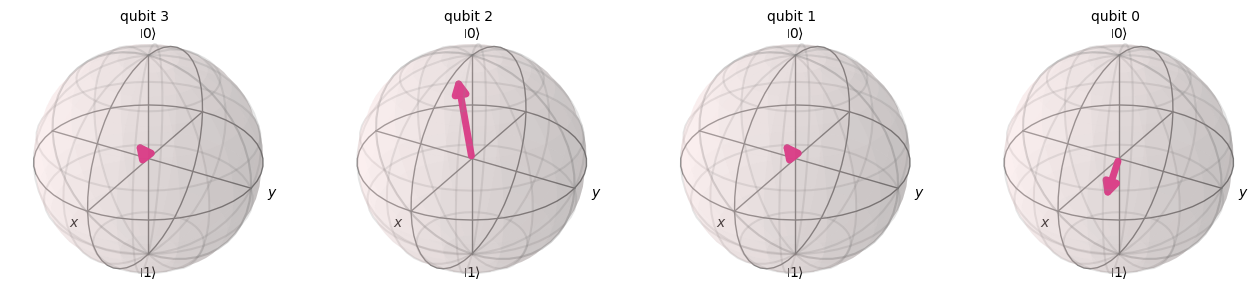Bloch sphere representation of density matrix

Hinton Plot

Hinton plot represents the real and imaginary parts of $n$-qubit state(s) on 2D plots by using squares. Positive and negative values are represented by white and black squares respectively, and the size of each square represents the magnitude of each value.

  
# Hinton plot of density_matrix
density_matrix.draw("hinton")

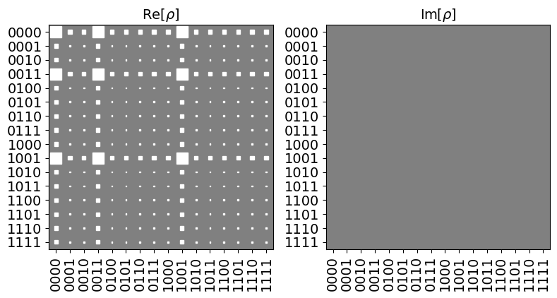Hinton plot representation of density matrix

Q-Sphere

Q-Sphere is a visualization of $n$-qubit state(s) that associates each computational basis state with a point on the surface of a sphere. A node is visible at each point; each node’s radius is proportional to the probability $p_{k}$ of its basis state, whereas the node color indicates its phase $\varphi_{k}$. The sphere’s north and south poles correspond to basis states $\ket{0}^{\otimes n}$ and $\ket{1}^{\otimes n}$ respectively, with all other basis states in between. Beginning at the north pole and progressing southward, each successive latitude has basis states with a greater number of $1$’s; a basis state’s latitude is determined by its Hamming distance from $\ket{0}^{\otimes n}$. The vector(s) on the sphere represents the system’s density matrix.

  
# Q-sphere representation of density_matrix
density_matrix.draw("qsphere")

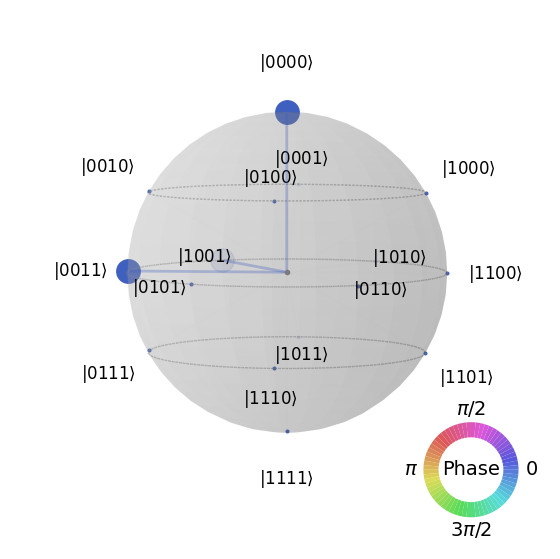Q-sphere representation of density matrix

References

article, quantum-computing

This post is licensed under CC BY 4.0 by the author.